Block caving: How to select the best multi-lift extraction level for maximum return

D Villa, J Romero and N Soto, Dassault Systèmes

23 Oct 2022 · 1500 words, 6 min read

In a block-caving project, the location of the extraction level is one of the most important decisions.

To a large degree, this decision defines project timing, capital costs, and resource recovery, and could eventually also expand maximum production capacity.

Determining the best extraction level for a single lift is complex. Deciding where to make multiple lifts is even more complicated.

To find an answer to the challenge of multiple lifts, we explored a number of options, finally landing on a combination of technologies that analyse the size and location of each lift based on thousands of scenarios using variable cut-off grades and production rates, while also employing fundamental financial KPIs and applying the ‘hill of value’ optimisation technique. The result: increased confidence that the extraction levels selected for multiple lifts will ensure not only maximum production capacity, but also maximum financial return.

Locating the extraction level for a single lift

The primary challenge for any lift is to try to predict or schedule the ‘best’ tonnages to extract from several draw points located in the extraction level for various periods, incorporating variables such as mining sequence, production rate, rate of opening new draw points, extraction rates, depletion method and many more.

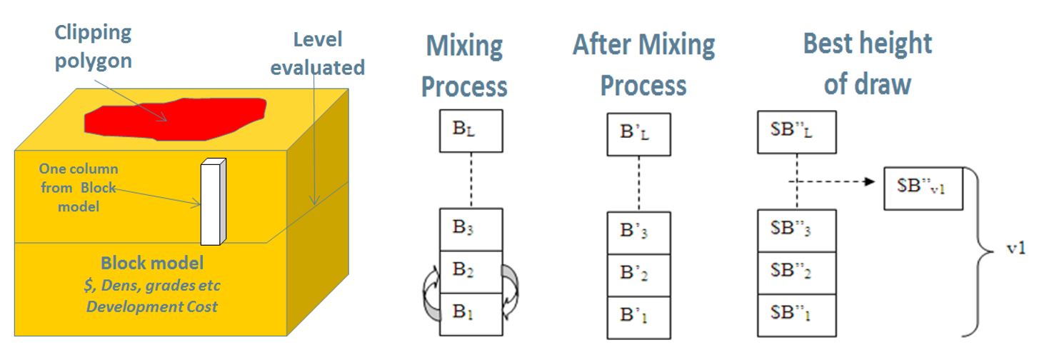
Existing technology, such as GEOVIA Cave Footprint Optimizer (formerly known as Footprint Finder), can generate a quick study using a block model to find the optimal extraction level elevation. The system evaluates all blocks inside a clipping polygon for each level selected. Each block represents one draw point, from which the system creates a draw column where it applies Laubscher's mixing method. From there, it calculates the best height of draw based on an economic evaluation that maximises the value using a vertical discount rate.

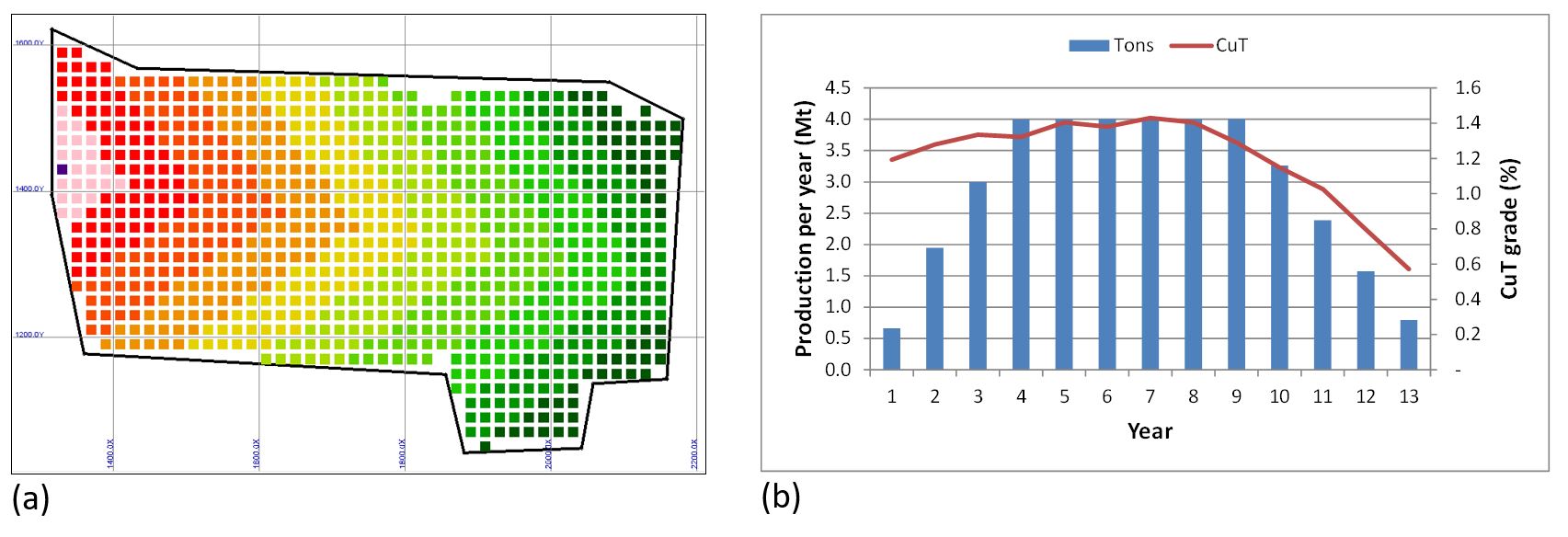
Figure 1: Footprint Optimizer’s evaluation steps.

Footprint Optimizer then takes the extraction for every level to simulate a production schedule using additional inputs, such as mining sequence (Figure 2a), production rate, numbers of new draw points, and extraction rates. From that schedule, it forecasts evaluation, tonnage, and grade by year (Figure 2b), and estimates the economic value of that level by considering the discount rate and (optionally) a capital cost.

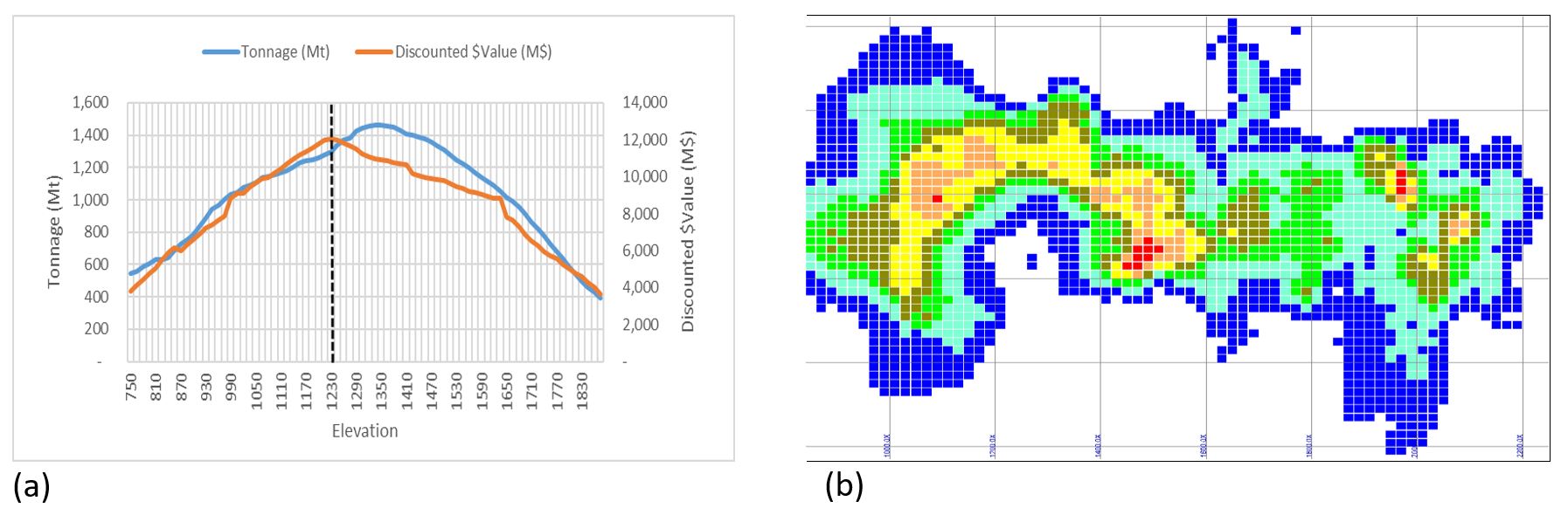
Figure 2: Production schedule in Footprint Optimizer: (a) mine sequence, (b) tonnage and grade.

After every level is evaluated economically, Footprint Optimizer summarises the results in various ways. Figure 3a, for example, compares tonnage and discounted cash flow, while Figure 3b displays the economic value by level and block.

Figure 3: Results from the Footprint Optimizer: (a) footprint size and (b) value distribution.

Locating the extraction level for multiple lifts

However, while Footprint Optimizer is very useful for identifying the best location of an extraction level for a single lift, it is not as useful for finding the optimum solution for more than one extraction level, owing to the complexity and number of possibilities that must be modelled. For multiple lifts, we tried to find a better solution by assessing three options:

Option 1: Select Lift 1, replace the grade above with the default value, then select Lift 2

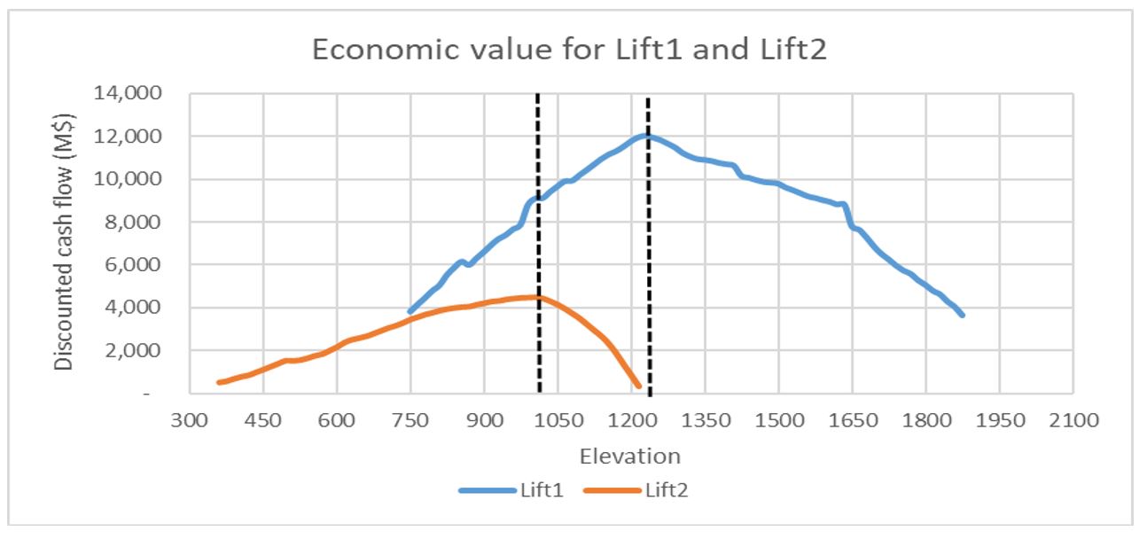
This option prioritised the selection of Lift 1 based on Footprint Optimizer’s usual initial inputs. Then, all blocks above Lift 1 by a default value are automatically replaced by null grade (assuming depleted material), to create a second analysis to find the best elevation for Lift 2. Figure 4 shows that, for this mine, the best combination of lifts would be Lift 1 at 1230 m, and Lift 2 – which represents only 30 per cent of Lift 1 – at 1000 m. However, the topography dictates that Lift 1 would be constructed at more than 1 km deep, meaning this option requires a high initial capital cost and a long lead-time to initiate production.

Figure 4: Option 1 selection of multi-lift elevation.

With this less-than-ideal result, we decided to look for an option that could determine the optimum location of the extraction level using a combination of both Lift 1 and Lift 2, but not necessarily establishing the location of Lift 1 first, followed by Lift 2.

Option 2: Assess Lift 1 and Lift 2 together, with the second lift at a given fixed vertical distance below Lift 1

Option 2, also using the standard Footprint Optimizer approach, assessed Lift 1 and Lift 2 together. However, because we did not yet know the elevation of Lift 1, we could not simply edit the block model to take into account the mining of Lift 1, so we placed the second lift at a fixed vertical distance below the base of Lift 1.

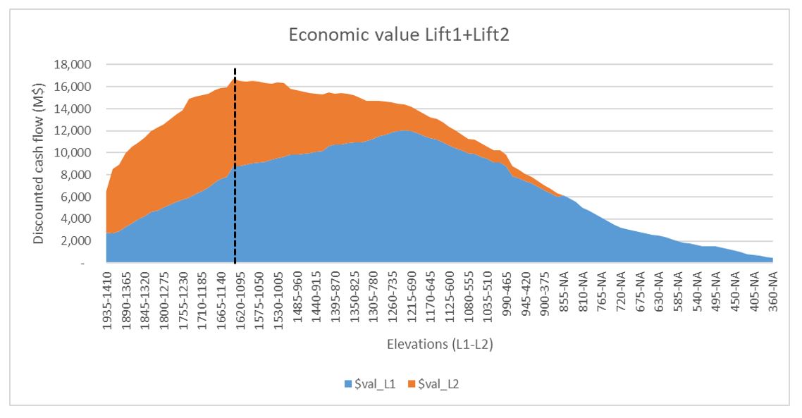
Figure 5: Option 2 selection of multi-lift elevation with a fixed vertical distance of 525 m. Please note that all discounted values are referred to the same year to make each combination valid as full NPV — Lift 1 + Lift 2 — and all combinations are directly comparable.

Option 2 successfully identified the best combination of both lifts by adding the value of Lift 1 and Lift 2, but we realised that a fixed vertical distance was not necessarily the optimal vertical distance. We needed the ideal combination of optimum Lift 1 elevation versus optimum Lift 2 location to determine the optimal vertical distance of the second lift.

Option 3: Assess Lift 1 and Lift 2, using scenario simulation and financial KPIs

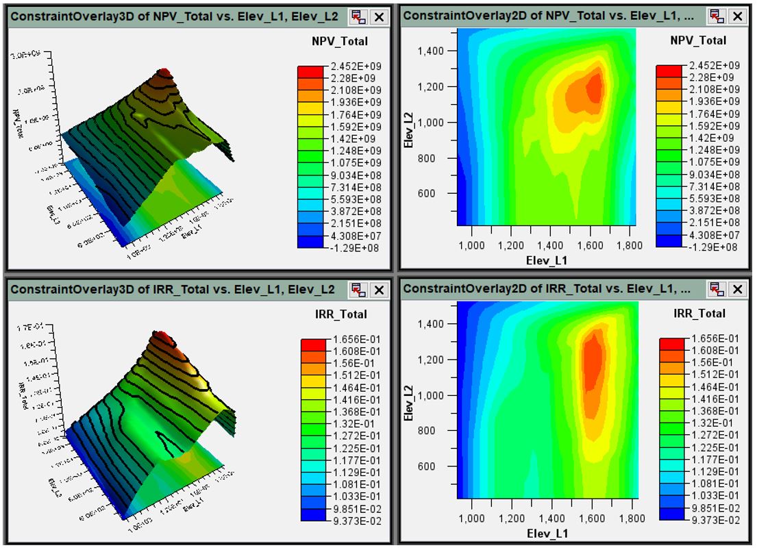
For Option 3, we used SIMULIA Isight in combination with the Footprint Optimizer, which allowed us to simulate a wide range of possible scenarios with specific (not standard) inputs, constraints, and engineering considerations. We also added in two financial KPIs as inputs — Net Present Value (NPV) and Internal Rate of Return (IRR), though other indicators like capital cost could be used as well — and applied the ‘hill of value’ optimisation technique, where the cut-off grade and the production rate are optimised in conjunction with obtaining the maximum NPV and IRR.

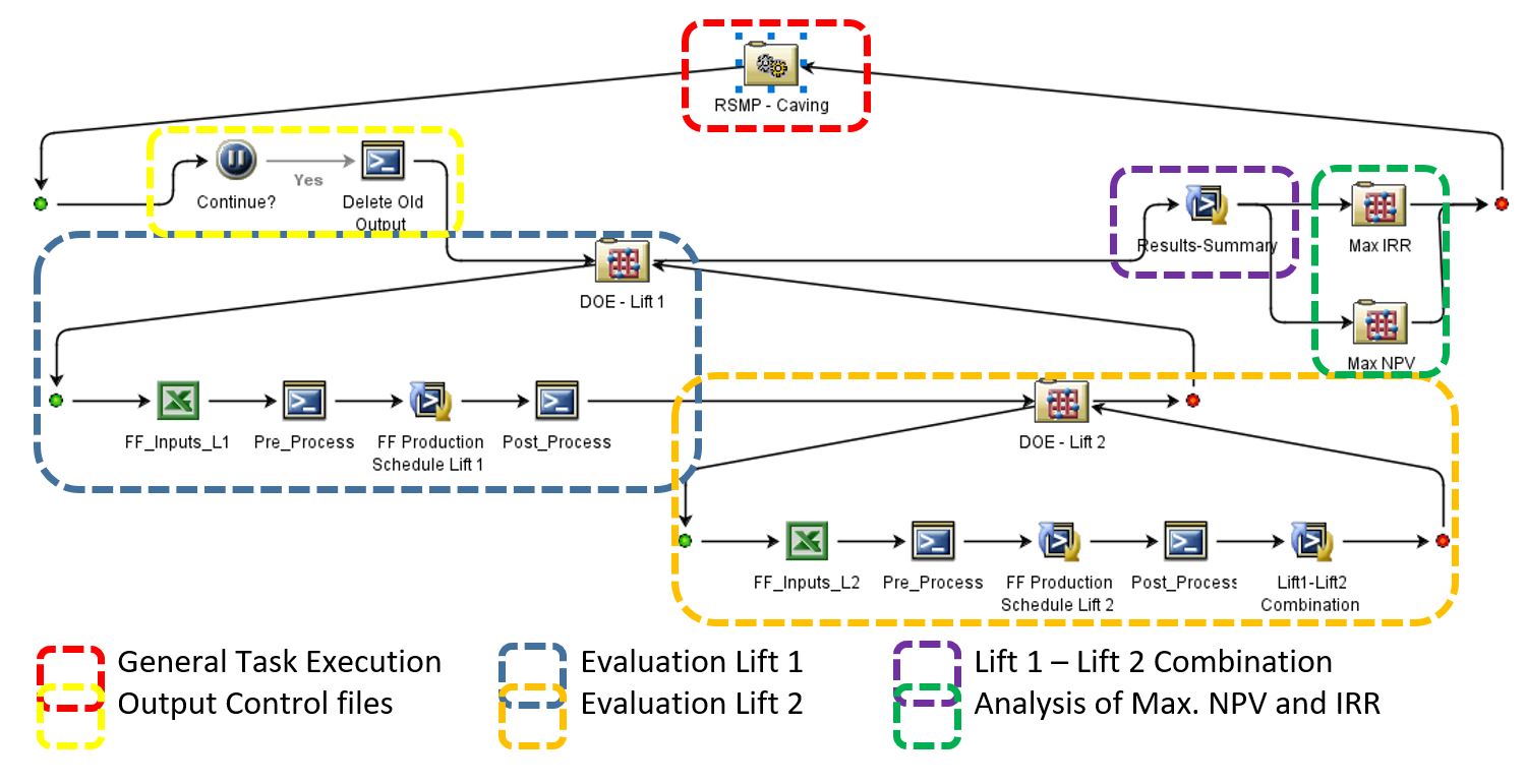
Figure 6: Footprint Optimizer and Isight workflow for multi-lift analysis.

To select the best elevation for Lift 1, our Design of Experiment (DOE) - Lift 1 had Footprint Optimizer simulate multiple scenarios while changing inputs such as production target, cut-off grade, capital cost, mine sequence, mixing parameters, development rate, etc.
Our DOE - Lift 2 evaluated Lift 2 in light of the results of DOE - Lift 1. For example, if Lift 1 was modelled at 500 m depth, every block above was replaced by null grades, assuming they would be extracted from Lift 1, and Lift 2 was evaluated from 500 m below for every level creating combinations such as L1:500 m & L2:550 m; L1:500 m & L2:600 m; L1:500 m & L2:650 m, etc.
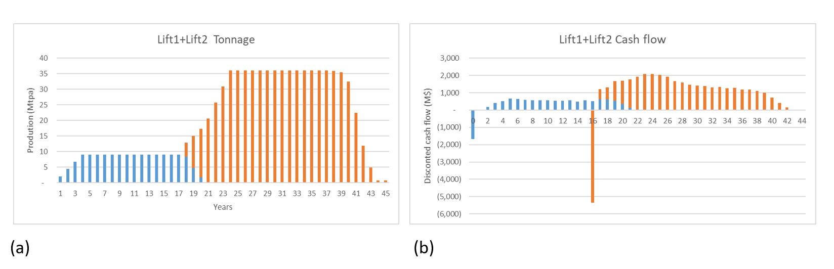
Footprint Optimizer then took the extraction for every level to first simulate a production schedule that assumed Lift 2 production would start as soon as the Lift 1 ramp-down started, and then forecast evaluation, tonnage, and grade by year for Lift 1 and Lift 2 in combination.
From there, Isight automatically calculated the cash flow per period and allocated capital cost at the beginning of each lift using a Python code that allowed us to explore different scenarios and apply different rules (see Figure 8). For example, we could:
- control the time for Lift 2 starts by an offset depending on the production target used by Lift 1, and
- apply a delay in production to replicate the additional development required to produce the first ore if the footprint analysed is located in deeper conditions — an option that helps associate the level location with the economic value calculated using NPV and IRR for each scenario simulated.

Figure 7: Option 3 Lift 1 and Lift 2: (a) production rate and (b) cash flow calculation.

Next, Isight reported tonnage, grade, and financial results (NPV and IRR) for every combination of Lift 1 and Lift 2, based on elevation, production target, and cut-off grade.
Finally, to analyse and select the best option out of thousands of scenarios, Isight:
- grouped the lifts into pairs, combining the elevation for each lift
- selected the pair with the highest NPV and IRR, and
- applied the hill of value optimisation technique to select zones with the best results (Figure 8).

Figure 8: Hill of value of NPV and IRR for Lift 1 and Lift 2.

Results

By simulating scenarios based on production target, cut-off grade and capital cost, Option 3 demonstrated improved discounted cash flow, reduced capital costs, and increased shareholder return. It also revealed options we had not initially envisioned, providing feasible and attractive alternatives for footprint size, mine plan and strategic mine design.

In short, Option 3 is a new technique that:

provides the ability to tie separate mining areas together, including multi-lift residual improvements
flows together multi-lift evaluation, production scheduling, and economic KPIs
automates the analysis of thousands of scenarios with built-in optimisation logic, and

enables good decision-making long before the detailed work is done.